One Way Anova Test

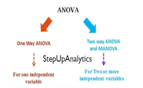
Anova means Analysis of Variance. One Way Anova is an important statistical test which is part of Hypothesis Testing and is generally done in the Analyze stage of Six Sigma project. It is used when there is one Continuous factor and one Discreet (generally categorical) factor.
One Way Anova checks the mean of all sub-groups present in the factor and verifies whether mean of all the sub-groups are equal or there is some difference in at least mean of one subgroup and rest of the subgroups.

Assumptions for One Way Anova test
1. Randomness: Data should be random and independent.
2. Normal Distribution: Data should be normally distributed.
3. Equal Variance: There should be equal variance or at least near about equal

How to fulfill these assumptions:
1. Randomness: For checking randomness of data, Run Chart would have to be used. If the P-value of all the 4 outputs – Clusters, Oscillation, Mixture and Trends is greater than 0.0. Then it means that data is random and independent.
2. Normal Distribution: Normality Chart would have to be used to check normality of data. If the P-value is greater than 0.05, then the data is normal. The P-value is also visible in Graphical Summary.
3. Equal Variance: Whether variance is equal or not can be checked through the Test of Equal Variance.

Minitab Navigation -> Stat – ANOVA – One way
(This option runs when our factor is comprised of stacked data)

Stat – ANOVA – One way (unstacked)
(This option is viable when our factor is comprised of unstacked data)

We will here use the stacked data option test:
Minitab -> Stat – ANOVA – One way
1. Select Y (Continuous value) in ‘Response’
2. Select x (Discreet value) in ‘Factor’
3. Press ‘Ok’
The resultant output is like this:

One-way ANOVA: A

HT versus Team Leader

Source DF SS MS F P
Team Leader 4 460303 115076 1.55 0.188
Error 540 40207340 74458
Total 544 40667643

S = 272.9 R-Sq = 1.13% R-Sq(adj) = 0.40%

Individual 95% CIs For Mean Based on
Pooled StDev
Level N Mean StDev —-+———+———+———+—–
Binny 110 442.2 289.3 (———*———-)
Jai 108 380.9 230.5 (———*———)
Ravi 112 386.1 266.5 (———*———)
Shishir 103 441.4 303.3 (———*———-)
Sunny 112 380.3 270.7 (———*———)
—-+———+———+———+—–
350 400 450 500

Pooled StDev = 272.9

Source – Two outputs are given :
• Factor ‘x’ (Discreet value) having subgroups. Here, Team Leader is x
• Error
DF – Degree of Freedom.
• Calculated for factor as( n-1), where n is No of Subgroups
• Calculated for Error as (n-DF for factor) where n is no of observations
• Total – DF for factor + DF for Error
SS – Sum of Squares – It represents the total variation in the data
• SS of factor – It measures the deviation of mean of factor levels and overall mean
• SS of Error – It measures the deviation of each data point from its factor level mean
• Total – SS of factor + SS of Error
MS – Mean Squares
• MS of factor = SS of factor/DF of factor
• MS of Error = SS of Error/DF of Error
F value = MS of factor / MS of Error
P-Value – Probability value to check whether Mean of all subgroups are equal or not
S – Square root of MS of Error
R-sqr – (SS Error/ SS Total) * 100
R-sqr (adj) – (MS Error/ (SS Total/DF Total)) * 100. MS Error is numerator and SS of Total divided by DF of Total is denominator
Level – Different level (group) in factor
N – Number of observations for each level of factor
Mean – Mean of each level of factor
StDev – Standard Deviation of each level of factor
Individual 95% Confidence Interval for Mean based on Pooled Stdev – It gives Individual Confidence Interval for Mean with 95% probability for all levels of factor