Process Capability for Non Normal Data

Process Capability for Non Normal Data is important subject for practitioners.

While accessing Process Capability for Non Normal Data it is critical that we identify what distribution is the data following. This is the critical first step for the subject at hand.

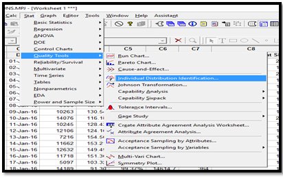
Step1: Check the distribution of the data which is under consideration.

Process Capability for Non Normal Data

Process Capability for Non Normal Data2

You can use Individual Distribution Identification functionality to perform capability analysis when the distribution of your data is unknown. The validity of statistics depends on the validity of the assumed distribution.

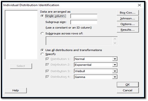
Use Individual Distribution Identification to compare the fit of up to 14 distributions and 2 transformations: normal, Box-Cox transformation, lognormal, 3-parameter lognormal, gamma, 3-parameter gamma, exponential, 2-parameter exponential, smallest extreme value, largest extreme value, logistic, log logistic, 3-parameter log logistic, Weibull, 3-parameter Weibull and Johnson transformation. The two transformations can be used to correct non normality in data

Minitab provides both graphical (probability plots) and numerical (goodness-of-fit statistics) output for comparison. The quantitative output also includes the estimates of the distribution parameters and percentiles for each distribution.

Process Capability for Non Normal Data4

Process Capability for Non Normal Data3

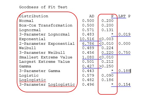
Check for the value which is closest to 1. That would be the likely distribution your data is following.

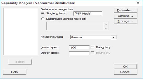
Process Capability for Non Normal Data5

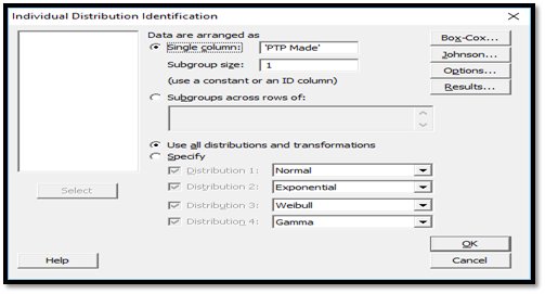
Put in the values that you have for the metric under consideration.

Process Capability for Non Normal Data6

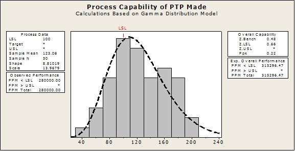
This is the result you shall receive.

The histogram of measurements consists of the following:

• A distribution curve that is superimposed on the histogram. The curve is the density function based on the estimated or specified parameters of the non-normal distribution used in the analysis. Compare the curve to the bars to assess whether the data are close to the distribution used in the analysis.
• Lower and upper specification limits (LSL and USL) represented by the vertical lines on the histogram. Compare the histogram bars to the lines to assess whether the measurements are inside the specification limits.